
Time Complexity on Single Source Shortest Path Algorithms
Published:
Graph data-structure is widely used represent different aspects in computer science (e.g., road network). We can denote the graph as \(G = (V, E)\), where \(V\) represents the set of vertices (in the context of road network it represents the intersections), and \(E\) represents the set of edges (in the context of road network it represents the road segments). Generally we define \(n~(= |V|)\) is the number of vertices and \(m~(= |E|)\) the number of edges to express the time and space complexity for algorithms related to graphs. One such problem is single-source shortest path (SSSP) that used to find the shortest path from a single node to all other nodes. For decades, Dijkstra’s algorithm has been the go-to method to solve this problem. The runtime of Dijkstra’s algorithm depends on the priority queue implementation and often has complexity of \(O(m + n \log n)\).
The new Algorithmic Breakthrough [Refer: Arxiv]
Recently, researchers proposed a new algorithm that challenges the long-standing dominance of Dijkstra. The key highlight, is reduced complexity of the new algorithm with computational complexity of
\[O\big(m \cdot \log^{2/3} n\big)\]This is strictly better asymptotically than Dijkstra’s \(O(m + n \log n)\) bound, especially for sparse graphs where \(m\) is closer to \(n\).
We could express the time complexity using simple functions as follows:
- \(O(n \log n + m)\) may be actually take \(k_1 \cdot n \log n + k_2 m\) computational units, where \(k_1,k_2\) are problem independent constants
- \(O(m \log^{2/3} n)\) may be actually take \(k_3 \cdot m \log^{2/3} n\) computational units, where \(k_3\) is problem independent constant
In order to make the new algorithm efficient we need to identify the maximum value of \(m\) such that the proposed approach outperforms the Dijkstra. Accordingly, we could formally express the inequality to detemine the maximum value of \(m\) as follows:
\[k_1 \cdot n \log n + k_2 \cdot m > k_3 \cdot m \log^{2/3} n\]Accordingly, \(m\) should satisfy the below constraints such that new approach to outperform the Dijkstra algorithm
\[m < \frac{k_1 \cdot n \log n}{k_3 \cdot \log^{2/3} n - k_2}\]For simplicity let assume all the problem indenpendent constants as \(1\), accordingly we can consider the simplified inequality, Accordingly, \(m\) should satisfy the below inequaltity such that new approach outperforms the Dijkstra algorithm:
\[m < \frac{n \log n}{\log^{2/3} n - 1}\]Refer the picture below which show how number of edges (\(m\)) varies for various node values (\(n\)),
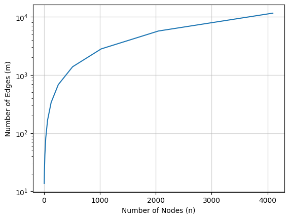
We observe that around \(n = 1000\), the \(m \approx 2744\). Above figure can be obtain from following code,
import math
import matplotlib.pyplot as plt

node_values = [2 ** k for k in range(2, 13)]
edge_values = []
for n in node_values:
    edge_value = n * math.log(n, 2) / (math.pow(math.log(n, 2), 2/3)  - 1)
    edge_values.append(edge_value)

plt.plot(node_values, edge_values)
plt.grid(which="major", alpha=0.5, linewidth=1)
plt.yscale('log')
plt.xlabel('Number of Nodes (n)')
plt.ylabel("Number of Edges (m)")
plt.show()
We could define the density of graph \(G\) by \(Den(G)\) as follows: \(\frac{2m}{n \cdot (n + 1)}\), which provides the ratio between the number of edges in the graph (\(m\)) and the number of edges possible based on the fact if all the nodes has an edge to all the other node (i.e., \(\frac{n \cdot (n + 1)}{2}\)).
Accordingly, we could replace the \(m = \frac{Den(G) \cdot n \cdot (n + 1)}{2}\), in the above inequality to find the relationship between maximum allowed graph density for a given node values,
\[\frac{Den(G) \cdot n \cdot (n + 1)}{2} < \frac{n \log n}{\log^{2/3} n - 1}\]Moving all \(n\) (\(n \geq 1\)) to right-hand side, we obtain the following inequality,
\[Den(G) < \frac{2 \cdot \log n}{(n + 1) \cdot (\log^{2/3} n - 1)}\]Refer the picture below which how maximum graph density (\(Den(G)\)) varies for various node values (\(n\)).
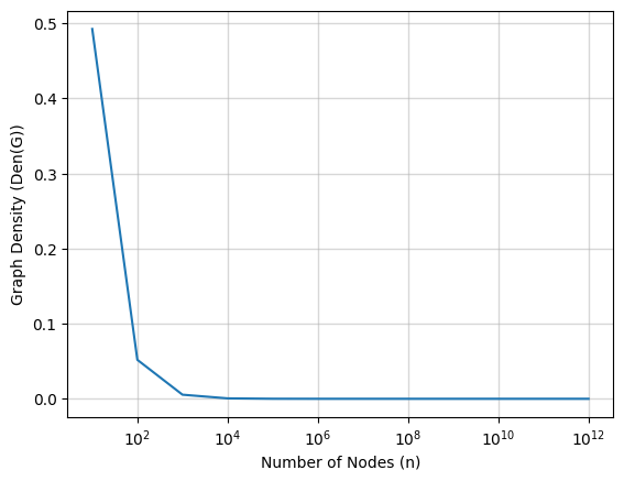
We observe that around \(n = 1000\), the \(Den(G) \approx 0.0055\) and \(m \approx 2744\), this signals, how sparse a network need to be inorder to achieve better performance using the new algorithm compare to Dijkstra. Above figure can be obtain from following code,
import math
import matplotlib.pyplot as plt

node_values = [10 ** k for k in range(1, 13)]
density_values = []
for n in node_values:
    density_value = 2 * math.log(n, 2) / ((n + 1) * (math.pow(math.log(n, 2), 2/3)  - 1))
    density_values.append(density_value)

plt.plot(node_values, density_values)
plt.grid(which="major", alpha=0.5, linewidth=1)
plt.xscale('log')
plt.xlabel('Number of Nodes (n)')
plt.ylabel("Graph Density (Den(G))")
plt.show()
This is generally reasonable for road networks, where not every node (i.e., intersection) is connected to every other node via road segments. In practice, most intersections connect to only a handful of nearby roads, making real-world road networks sparse graphs. This sparsity is exactly why proposed new algorithm with time complexity of \(O(m \log^{2/3} n)\), can yield reasonable performance gains over Dijkstra, especially as the network scales to tens or hundreds of thousands of nodes. For an example in Chattanooga, TN the road network from OpenStreetMap has road-network with \(n = 10,788, m = 28,100\) (Refer: Paper), based on the above expression the \(m\) can go upto \(31,142\). Note that, we simplified the inequality where we let all the independent constants $k_1,k_2,k_3$ to be equal to 1, so this evidence may not sufficient enough to support above claim.